
3point.xyz


In this article, you will learn how to pinpoint where fires occur anywhere, create composite satellite imagery before, during, and after fires, calculate normalized burn ratio, and quantify burn severity areas.
PREREQUISITES
Google Earth Engine Account, working coding knowledge, and general GEE platform functions. For a beginner's tutorial, refer to Chapter 2 of the FOSS resources. For an introduction to remote sensing read the first chapter of the Earth Engine Fundamentals text.
FIRES
Fires in Serengeti and Masai Mara National Parks have burned massive areas this year. With Google Earth Engine, it's possible to quantify burn severity using the normalized burn ratio function and then calculate the total area burned by classification areas.
WORKFLOW
A typical workflow for this analysis would be the following:
- Select study area, time frame, and datasets
- Apply a cloud-mask algorithm to pre- and post-fire image collections
- Create cloud-free composites
- Calculate Normalized Burn Ratio for pre- and post-fire dates
- Calculate dNBR by subtracting pre- and post-NBR imagery
- Classify burn severity classes
- Quantify burn severity class areas and % areas
- Visualize results
However, we will modify this workflow slightly by organizing the code into sections to group similar functions, and then visualize and classify the results.
GEE
Google Earth Engine (GEE) has access to petabytes of planetary data, ready for use in remote sensing analyses. It is excellent for exploring datasets when you begin a project, regardless of what geospatial platform you normally use. You can use your Google account to set up a GEE account.
EDA
Let's begin with some exploratory data analysis, also known as EDA. Outside the United States, fire burn perimeters are not easily accessible. Let's examine NASA's VIIRS radiometry imagery to gain insight into recent burns in the general region we want to study, also known as an area of interest (AOI). In the search bar at the top of the GEE console, enter NASA VIIRS fire and select the first raster dataset that appears with NOAA. In the new open window, read through the dataset documentation. VIIRS picks up radiation from Earth's surface, resulting in visible hotspots. Generally, these hotspots correlate with fires. On the left-hand side of the window, click see examples. A new GEE window will open.
Click run to check out the example. Presto! You don't even need to know JavaScript to check out the dataset. However, the console zooms you near Lake Athabasca in Canada, and the data is from 2023. Let's modify the script to zoom into the Serengeti and focus on imagery from January to March 2025.
I've modified the original code to make it more readable, and added some comments (indicated by the double backslash) to explain the code. Comments are lines that are not processed when the code is run.
// Import NOAA VIIRS satellite imagery and filter to Jan-March 2025
var viirs = ee.ImageCollection('NASA/LANCE/NOAA20_VIIRS/C2')
    .filter(ee.Filter.date('2025-01-01', '2025-03-17'));

// Create the visibility parameters
var vis = {
  min: 280,
  max: 400,
  palette: ['yellow', 'orange', 'red', 'white', 'darkred'],
  bands: ['Bright_ti4'],
};

// Center map and zoom then add layer and name
Map.setCenter(34.845, -2.166, 8);
Map.addLayer(viirs, vis, 'Serengeti Fires 2025');
Running the newly modified code results in the following map of northern Tanzania, showing Serengeti and Masai Mara National Parks in darker green and the red and yellow pixels indicating fires. After running the code, a new layer called 'Serengeti Fires 2025' appears in the layers pull-down box.
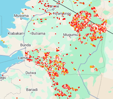
We can see from the resulting map that a cluster of fires is located along the Kenyan-Tanzanian border, where the two parks meet. However, most of the fires appear to be situated on the Serengeti National Park side in Tanzania.
Let's examine this code in a little more detail:
- JavaScript assigns variables using 'var' plus the variable name. In the first line, we create the variable viirs and assign it to the NASA VIIRS image collection. This imports the dataset into our analysis.
- In the second line, we use the .filter command to tell JavaScript to select imagery from January to March 2025 in yyyy-mm-dd format. The filter function is useful for other filtering within the dataset, such as satellite band selection.
- You will notice alternating capitalization of letters in the commands. This is known as Camel Case and is used in many programming languages. It doesn't make remembering commands easy. Still, you can always cut and paste from the code documentation, look up solutions online, such as GIS Stack Exchange, or ask an AI chatbot to help you develop code. And the more you use it, the easier it becomes to remember what is capitalized or not.
- The second section sets up the visibility parameters for the satellite imagery, sometimes referred to as 'vis' or 'vis params'. The min/max values are typically derived from the dataset documentation. I removed the brackets and extra decimal places from the example as they were superfluous.
- The last commented section centers the map using latitude, longitude, and a zoom value. The last line adds the data to the map with the vis params and specifies a name for the new layer. To get the latitude/longitude (lat/lon) in Earth Engine. Zoom to your area of interest, click the inspector in the upper right panel, click where you want the map to center in the map console, copy and paste the lat/lon from the inspector into the parentheses with the `Map.setCenter` command.
This workflow is typically how you would start, e.g., import the dataset, set the visibility parameters, and add the map to the console.
AOI
Now that we've conducted some EDA to determine where we want to focus the analysis, let's create an area of interest. From the VIIRs data, we saw wildfires in the Masai Mara National Reserve and Serengeti National Park. Using the handy polyline tool, I selected the four corners of a polygon (there are five total lines; the last line is the same as the first to close the polygon) and copied them into the code block. You can also copy the code between the curly brackets in the polyline tool and assign that to a variable (kinda messy), or use the shape drawing tools in the upper left corner of the Earth Engine map panel.
// ==========================
// 1. Define AOI and Constants
// ==========================
var aoi = ee.Geometry.Polygon([
    [34.59479472180698, -1.8712263041221182],
    [35.47370097180698, -1.8712263041221182],
    [35.47370097180698, -1.305650124406412],
    [34.59479472180698, -1.305650124406412],
    [34.59479472180698, -1.8712263041221182]
]);

var visParams = {
    min: 0.0,
    max: 0.3,
    bands: ['B4', 'B3', 'B2']
};

var severityVisParams = {
    min: 0,
    max: 4,
    palette: ['green', 'yellow', 'orange', 'red', 'magenta']
};

var severityClasses = ['Unburned', 'Low', 'Moderate-low', 'Moderate-high', 'High'];
var severityValues = [0, 1, 2, 3, 4];
The second part of this section adds the visibility parameters for the imagery and the severity mapping (visParams and severityVisParams variables). The last two lines assign values to dictionaries of the severity classes (severityClasses and severityValues).
NBR
The normalized burn ratio (NBR) is a spectral index that estimates burn severity (Roy et al., 2006). NBR is calculated using the following formula:
NBR = (NIR - SWIR) / (NIR + SWIR)
Where NIR = near infrared band and SWIR = shortwave infrared reflectance
The bands for the formula will change depending on the satellite data you're using. For Sentinel-2, Band 8 is NIR and Band 12 is SWIR. Be sure to review the documentation for each dataset you import to select the correct bands. Earth Engine has a handy NBR function, so for Sentinel-2 bands it is
image.normalizedDifference(['B8', 'B12'])We'll use this formula in the 'Functions' section, but first, we'll create a function that masks clouds and another that clips the satellite image collection to the AOI we created earlier.
// ==========================
// 2. Functions
// ==========================

//Masks clouds using the Sentinel-2 QA band.

function maskS2clouds(image) {
    var qa = image.select('QA60');
    var cloudBitMask = 1 << 10;
    var cirrusBitMask = 1 << 11;
    var mask = qa.bitwiseAnd(cloudBitMask).eq(0)
        .and(qa.bitwiseAnd(cirrusBitMask).eq(0));
    return image.updateMask(mask).divide(10000);
}

//Clips image collection to the AOI.

function clipCollection(collection) {
    return collection.map(function(image) {
        return image.clip(aoi);
    });
}

//Calculates NBR

function calculateNBR(image) {
    return image.normalizedDifference(['B8', 'B12']).rename('nbr');
}
The 'Load and Process Data' section loads and processes the data. We add the pre- and post-fire imagery from Sentinel 2, filter it to the appropriate dates, filter out cloudy pixels with a percentage less than 20%, and apply the cloud mask function. Then clip those images to our AOI. Clipping makes processing much faster and enables analysis at the pixel size level, as supported by Earth Engine. The final processing involves calculating the NBR and the change in NBR, or dNBR. The latter is simply subtracting the mean pre-imagery from the mean post-imagery.
// ==========================
// 3. Load and Process Data
// ==========================

// Load pre- and post-fire Sentinel-2 data
var preFire = ee.ImageCollection('COPERNICUS/S2_SR_HARMONIZED')
    .filterDate('2024-03-01', '2024-03-17')
    .filter(ee.Filter.bounds(aoi))
    .filter(ee.Filter.lt('CLOUDY_PIXEL_PERCENTAGE', 20))
    .map(maskS2clouds);

var postFire = ee.ImageCollection('COPERNICUS/S2_SR_HARMONIZED')
    .filterDate('2025-03-01', '2025-03-17')
    .filter(ee.Filter.bounds(aoi))
    .filter(ee.Filter.lt('CLOUDY_PIXEL_PERCENTAGE', 20))
    .map(maskS2clouds);

// Clip collections to AOI
var preFireClipped = clipCollection(preFire);
var postFireClipped = clipCollection(postFire);

// Calculate NBR and dNBR
var beforeNBR = preFireClipped.map(calculateNBR);
var afterNBR = postFireClipped.map(calculateNBR);
var dNBR = beforeNBR.mean().subtract(afterNBR.mean()).rename('dNBR');
VISUALIZATION
GEE is great at crunching calculations through complex datasets. The calculations happen in the cloud, so you can rapidly process and analyze large datasets on almost any computer. However, the platform is not so awesome at visualizing results. The 'Visualize' section adds map layers to the map console, creates burn severity classes for the dNBR data, and then adds the severity map.
// ==========================
// 4. Visualize
// ==========================
// Add layers to the map
Map.centerObject(aoi, 10);
Map.addLayer(preFireClipped.mean(), visParams, 'Serengeti Pre Fire');
Map.addLayer(postFireClipped.mean(), visParams, 'Serengeti Post Fire');
Map.addLayer(dNBR, {min: -1, max: 1, palette: ['white', 'black']}, 'dNBR');
// Classify burn severity
var severity = dNBR
.where(dNBR.lt(0.10), 0)
.where(dNBR.gte(0.10).and(dNBR.lt(0.27)), 1)
.where(dNBR.gte(0.27).and(dNBR.lt(0.44)), 2)
.where(dNBR.gte(0.44).and(dNBR.lt(0.66)), 3)
.where(dNBR.gt(0.66), 4)
.clip(aoi);
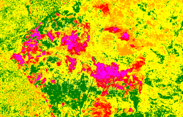
Map.addLayer(severity, severityVisParams, 'Burn Severity');Cool! That gives you four image layers:
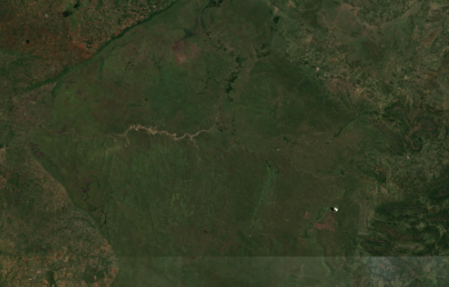
Prefire from 2024:
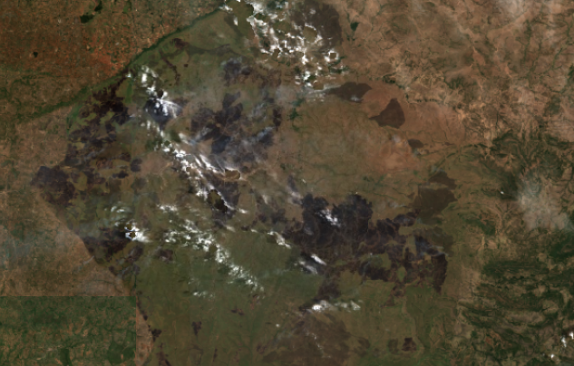
Jan to March 2025 during the fires. Note, there is some cloud or smoke cover that obfuscates the results and may create issues for the dNBR classification:
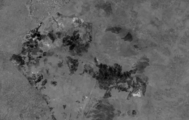
Unclassified dNBR:
Classified burn severity:
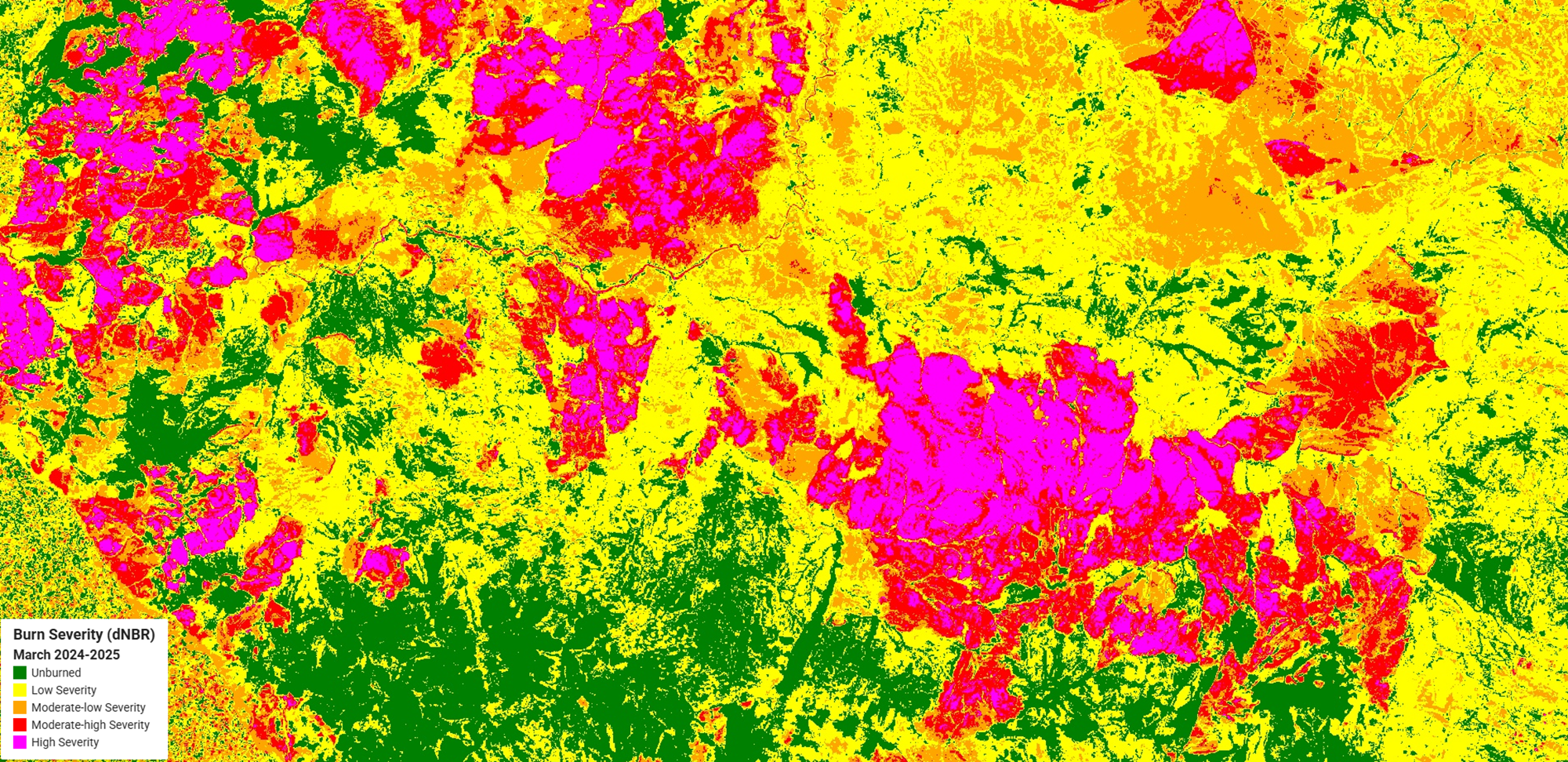
LEGEND
Adding map legends is not straightforward, but once you have the code, it can be reproduced with slight tweaks for other analyses and maps. This legend is 'only' 34 lines of code!
 // ==========================
// 6. Add Legend to Map
// ==========================

var legend = ui.Panel({
    style: {
        position: 'bottom-left',
        padding: '8px 15px'
    }
});

legend.add(ui.Label({
    value: 'Burn Severity (dNBR)',
    style: {fontWeight: 'bold', fontSize: '18px', margin: '0 0 4px 0', padding: '0'}
}));

legend.add(ui.Label({
    value: 'March 2024-2025',
    style: {fontWeight: 'bold', fontSize: '16px', margin: '0 0 4px 0', padding: '0'}
}));

var makeRow = function(color, name) {
    return ui.Panel({
        widgets: [
            ui.Label({style: {backgroundColor: color, padding: '8px', margin: '0 0 4px 0'}}),
            ui.Label({value: name, style: {margin: '0 0 4px 6px'}})
        ],
        layout: ui.Panel.Layout.Flow('horizontal')
    });
};

var palette = ['green', 'yellow', 'orange', 'red', 'magenta'];
var names = ['Unburned', 'Low Severity', 'Moderate-low Severity', 'Moderate-high Severity', 'High Severity'];

palette.forEach(function(color, index) {
    legend.add(makeRow(color, names[index]));
});

Map.add(legend);
Now we have the map with legend showing the dNBR classifications:
RESULTS
Generally, it appears that the highest severity areas of the burn are grass and scrub areas, with several areas of unburned coinciding with forest. But you can also see the heterogeneous nature of the fire, where it burns severely in some areas, skips others, or burns at a low to moderate intensity in others. This is due to weather patterns at the time and possibly suppression efforts. For increased accuracy, it may be wise to ground-truth the burn severity, especially in areas obscured by clouds or smoke. You may also need to find an image free of clouds or smoke. The algorithm we used in this instance did not remove clouds from the image.
AREA CALCULATIONS
That's all great, but what if you want to know how much of the fire in the AOI is high-intensity or not affected? We can sum the total pixels in the AOI using the .sum function, then count pixels by burn severity classes using the Reducer function. A common workflow for image processing is filter, map, and reduce (Cardile, 2023). Reducers are used in Earth Engine to aggregate data over time, space, bands, arrays, and other data and are often used to calculate image statistics.
This data can be manipulated to area and percent of total using .divide and .multiply functions. The 'Calculate Area Statistics' section calculates the total area in km², then calculates the severity class statistics, converting them to km² and percent of the total, then prints the results to the console.
// ==========================
// 5. Calculate Area Statistics
// ==========================

var pixelArea = ee.Image.pixelArea().clip(aoi);
var aoiPixelArea = pixelArea.reduceRegion({
    reducer: ee.Reducer.sum(),
    geometry: aoi,
    scale: 10,
    maxPixels: 1e9
}).get('area');

var aoiKm2 = ee.Number(aoiPixelArea).divide(1e6).round();
print('AOI area (km²):', aoiKm2);

var severityStats = severityValues.map(function(value) {
    var classMask = severity.eq(value);
    var classArea = pixelArea.updateMask(classMask).reduceRegion({
        reducer: ee.Reducer.sum(),
        geometry: aoi,
        scale: 10,
        maxPixels: 1e9
    }).get('area');

    var classKm2 = ee.Number(classArea).divide(1e6).round();
    var classPercent = ee.Number(classArea).divide(aoiPixelArea).multiply(100).round();

    return {
        class: severityClasses[value],
        area_km2: classKm2,
        percent: classPercent
    };
});

print('Severity class areas (km²):', severityStats);
severityStats.forEach(function(stat) {
    print('Class:', stat.class, 'Area (km²):', stat.area_km2, '% area:', stat.percent);
});
A summary of the severity class areas and % area is shown in the following table:
| Severity Class | Area (km²) | % Area |
| Unburned | 1,544 | 25 |
| Low | 2,728 | 45 |
| Moderate-low | 1,038 | 17 |
| Moderate-high | 505 | 8 |
| High | 302 | 5 |
| Total Area | 6,017 |
Despite the high severity class standing out on the map, it occupies the lowest percentage of the burn. This could also be due to the dominant grassland vegetation, e.g., grasses burn rapidly but are generally low-growing and are not classified as high severity. Again, it would be useful to examine various areas of the burn on the ground to see if the imagery matches reality.
LIMITATIONS
Approach results from any remote sensing analysis with a skeptical eye. Results are subject to false positives, and vice versa, or changes in vegetation, the vegetation type, and land cover may skew results or increase errors, especially if compositing images over long periods (UNSKP). Ground-truthing results are ideal and can be correlated with your analysis. However, ground truthing isn't always feasible due to staff capacity and availability. We have noted two instances where the imagery may have been obscured by clouds or smoke and where it appears that most of the fires are of low severity due to the predominant vegetation types. Correlating field observations with remote sensing analysis provides a powerful triangulation tool for making inferences at large scales.
CODE
The link to the full code is here. Please let us know if you are trying this, where your AOI is located, and what you find out!
1 May 2025 11:44am
This was originally presented on 24 April, 2025 as part of a Geospatial Group Cafe. We will post the recording and highlights from other speakers of that session soon!
Elsa Carla De Grandi
Fauna & Flora

10 June 2025 5:39pm
Thanks for presenting this during our Geospatial Cafe! Looks very useful!
I wonder if, to get rid or the haze, smoke and clouds you could try using the Harmonised Landsat and Sentinel-2 imagery instead as this is collected every 2 - 3 days or experiment a bit with the dates of the post-fire image to get rid of the smoke and clouds or perhaps use s2cloudless.
Also noting that it is possible to upload and import your own shapefile to GEE if you already have an Area of Interest (AOI) you want to look at without having to specify the polygon coordinates.
Harmonized Landsat and Sentinel-2 | NASA Earthdata
NASA's Harmonized Landsat and Sentinel-2 (HLS) project generates global land surface reflectance data every 2 to 3 days at 30 meter resolution.

Vance Russell
3point.xyz